Introduction

Two people who earn the same amount can face very different odds of hardship depending on the family they live in. Here’s why: The government sets the poverty line higher for bigger households, because they need more money to cover the basics. Kids raise that bar, but they don’t bring home a paycheck. Adults do. So it really comes down to two things: how many people are earning and how many are living on what those earners make. A married couple without children can have two paychecks covering the bills. A single parent usually has one — and more mouths to feed. A working grandparent under the same roof can help close the gap. That’s how the same wage can leave one family fine and another falling behind. It’s not just what a household earns, it’s how many are earning it and how many depend on it.

Among Chicagoans, who most likely lives below the poverty line?

The Illinois Policy Institute analyzed five years of U.S. Census microdata on metropolitan America. Chicago-area families live inside those national patterns, which are clear: The people most likely struggling to make ends meet are those raising children without a spouse in the home and households headed by someone who never finished high school.

One thread runs through every group at high risk of poverty: trouble getting — and keeping — full-time, well-paid work. Single parents stretched across one income, adults without a high school diploma, and young, recent arrivals — each meets the same wall from a different side: too few earners, too little earning power, or too little time in the labor market.

One thing to keep in mind: These traits tell us where people below the poverty line are concentrated, not necessarily that those traits cause poverty. The analysis can’t show how much having children, living without a spouse or not finishing high school by itself lowers a family’s ability to pay its bills with its own earned income. The data simply show that people below the line are far more likely to share these characteristics, which is what makes those characteristics useful for pointing help where it’s needed most.

Living with children and no spouse present: the group most likely to be below the poverty line

Two features of a household track most closely with poverty: whether it includes children and whether the head of the household has a spouse in the home. On their own, each is linked to a modest increase in likelihood that the household lives beneath the poverty line. Together, they mark the group most likely to be found below the line.

The intuition is straightforward. Every child in the home raises the income a family needs to stay out of poverty; more people to feed and house requires more money. A spouse in the home is a second potential paycheck: Two parents can split the earning and the childcare, while a single parent has to do both, often paying for childcare just to hold down a job. More need, fewer earners and a harder path to working — that’s the combination that pushes this group below the line.

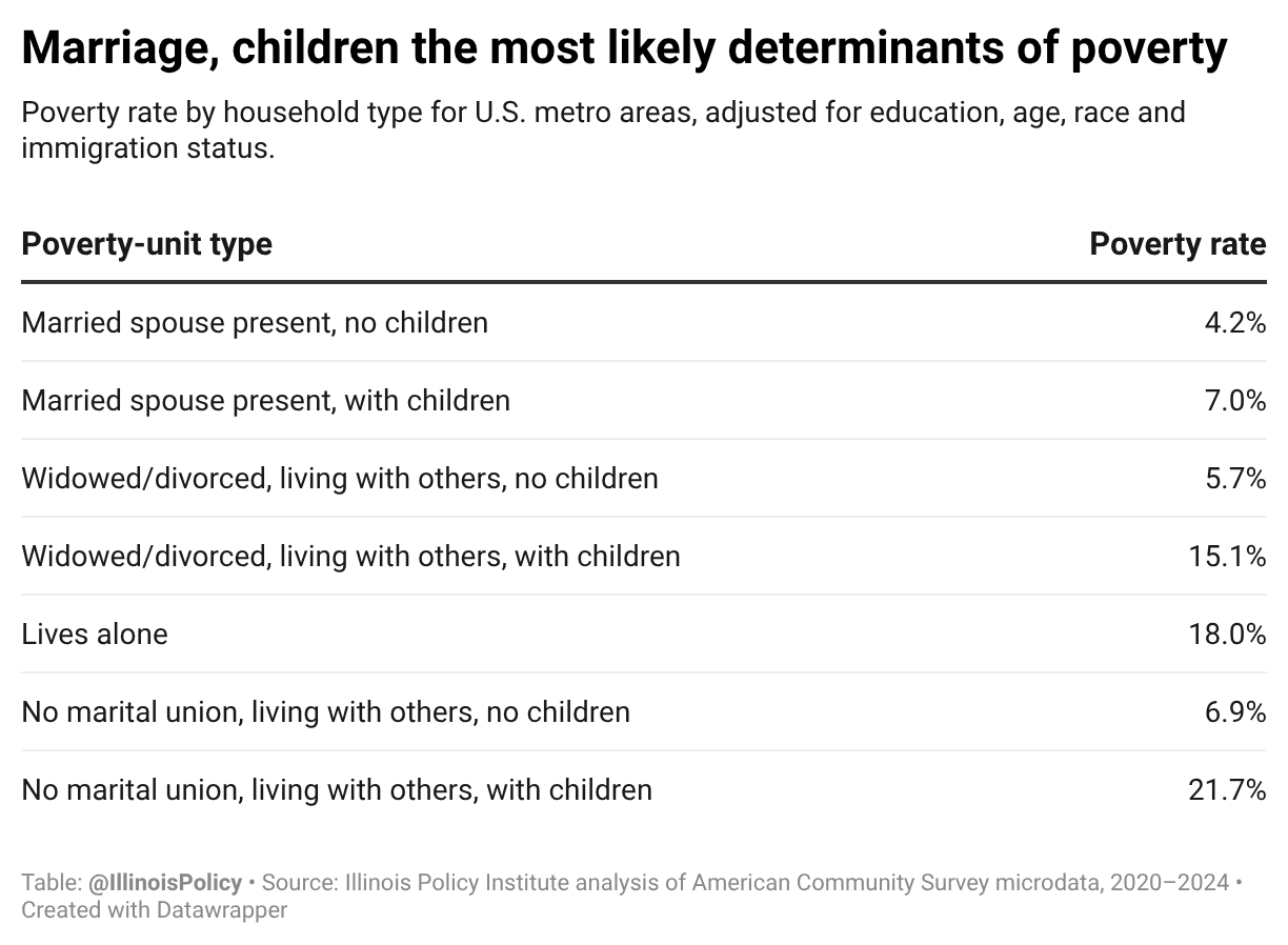
Adjusting for local housing costs and holding education, age, race and immigration status constant, the poverty rate in U.S. metro areas is 4.2% for married couples without children but 7% — nearly double — for married couples with children.

For households with no marital union and no children, the poverty rate is 6.9%. But when children are present with no spouse, it jumps to 21.7% — roughly one in five. Put another way, a child adds little to a married couple’s likelihood of finding themselves strapped for cash but significantly increases it for a single adult. That likelihood grows with each child. The poverty line rises every time a household adds someone, so a single parent raising three kids on one income has to earn far more to stay above the line than one raising a single child. For a married couple, a second paycheck absorbs much of that added cost, which is why kids don’t move their numbers as much.

Education matters just as much as family structure

Holding everything else constant, differences in schooling matter. The poverty rate is about 5.2% when the head of household has a bachelor’s degree or higher, but about 20.5% when that person did not finish high school.

This is nearly the same spread as the gap between a married couple with children and an otherwise-similar single-parent household. That is consistent with finishing high school raising employment and income, though people who finish high school may also differ in ways the data don’t capture.

Education is one of the few factors a family and a school system can act on before poverty takes hold.

Young families are the most exposed

Poverty risk is highest among households headed by younger adults. The risk falls through the prime working years and flattens out approaching retirement — the mirror image of the earnings curve. As people build skills and work experience, their incomes rise and their odds of poverty fall. The most vulnerable years are the early ones, when families are youngest and paychecks are smallest.

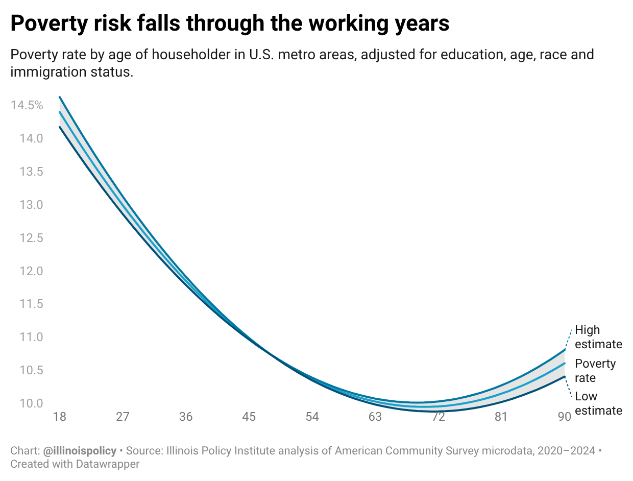
The poverty risk profile over the lifecycle is perhaps more suggestive evidence of the importance of work and earnings to avoid falling below the poverty line.

Race gaps narrow sharply once everything else is accounted for

When comparing households with the same education, age, family structure, immigration status and location, the gaps between racial and ethnic groups shrink.

The Hispanic-white gap nearly closes: 10.4% for Hispanic-headed households vs. 9.8% for white. The Black-white gap narrows but does not disappear: 13.1% versus 9.8%. Even accounting for everything else, Black-headed households are still more likely to be under the poverty line than similar white households. Those gaps can also reflect differences in employment and earnings — who’s working, how much, and at what wage — which the analysis doesn’t hold constant.

What Illinois can do

The analysis points to the importance of employment income. Research on social capital, such as relationships and community support, suggests it can help connect people to that income. Policies that support schooling and boost employment income, that reward attachment to work and that reinforce a stable local community would likely improve the conditions of Chicagoans living below the poverty line.

The groups most at risk here all struggle with the same thing: getting and keeping full-time, well-paid work. So the test for any policy is simple: Does it increase employment income or make it easier to find and keep a job, or does it raise income without changing a family’s ability to earn?

What treats root causes of poverty

One option is the federal Earned Income Tax Credit. It is a check, but paid only to people who work, designed to make taking a job pay off. Most research finds it drew more single mothers into work, though some economists dispute how large that effect was and how much it raised earnings over time. Sectoral training, which teaches skills for specific jobs local employers need to fill, has some of the strongest evidence of lasting earnings gains. Place-based investment can help, too, but only when it’s judged by whether the residents already there land better jobs at higher wages, not by how much money gets spent. Block clubs and other neighborhood groups earn their place as the connector — not the paycheck, but the on-ramp that links residents to employers, training and networks beyond the block.

Guaranteed-income payments, which are unconditional cash, eased hardship while they lasted in recent experiments, but recipients worked slightly less and their own earnings fell; when the money stops, so does the gain. The expanded 2021 Child Tax Credit worked the same way: It sharply cut measured poverty while it was paid, but that drop reversed once it ended. Traditional means-tested programs can also discourage earning when they’re built around income cutoffs, as a raise or a few more hours can cost a family its benefits. For working-age adults, these programs relieve hardship today but do little to change what a family can earn tomorrow. Children are the exception: Research finds that children whose families had access to food assistance and health coverage grew up healthier and more self-sufficient as adults.

The lesson is to build the effort around the things that can actually address root causes and be honest about what only alleviates the symptoms: Reward and enable work, invest early in children for the long run, and use community organizations to connect people to the jobs and training that actually move earnings.

Appendix: Data and methodology

Data sources and study population

This analysis uses person and housing records from the U.S. Census Bureau’s American Community Survey (ACS), accessed through IPUMS USA. All principal published estimates use the 2020–2024 ACS five-year sample. A separate, supplementary linear model pools that sample with the nonoverlapping 2015–2019 sample to examine metropolitan associations. The published local poverty lines and principal group comparisons use 2020–2024 data.

The population studied consists of ACS respondents in identifiable U.S. metropolitan areas for whom poverty status can be determined under the rules below. The results do not represent the entire United States. Local estimates are reported for metropolitan areas and Public Use Microdata Areas (PUMAs), the smallest areas identified in the ACS public-use microdata. The local estimates use 2020 PUMA definitions. Because the two ACS samples use different PUMA boundaries, their PUMA codes are not treated as comparable places across time.

Local prices are based on Bureau of Economic Analysis (BEA) metropolitan regional price parity components for rents, utilities, goods and other services, matched by survey year. Six metropolitan codes are mapped between the definitions used by IPUMS and BEA. Two areas classified as micropolitan under the newer definitions — East Stroudsburg, Pennsylvania, and Ocean City, New Jersey — lack a matching BEA metropolitan parity and are excluded from the cost-of-living-adjusted area estimates. Metropolitan names come from IPUMS geographic labels; PUMA names come from Census boundary files using 2020 PUMA definitions. The spending shares used to combine BEA components are informed by the Bureau of Labor Statistics Consumer Expenditure Survey.

Poverty units, income and the analysis sample

Poverty is assessed for a poverty unit, whose members share resources and a poverty classification. We reconstruct these units from the ACS household relationship records. The householder and related household members form one unit; each unrelated person aged 15 or older forms a separate one-person unit. Unrelated children under 15 are outside the poverty universe. We calculate poverty status using the reconstructed unit’s income and threshold because the family grouping supplied in the microdata does not always coincide with the poverty unit used here.

The ACS microdata do not provide a ready-to-use threshold for every reconstructed unit. We recover threshold amounts from records whose IPUMS family and reconstructed poverty unit coincide: family income is divided by the reported income-to-poverty ratio. We take the median recovered amount for each combination of survey year, unit size, number of related children under 18 and whether the reference person is at least 65. For a unit without an exact match, we use a threshold for the same year, size and age category averaged over child counts; if necessary, we use one for the same year and size averaged over age categories. Units for which no threshold can be recovered are excluded. The reconstructed unit’s income is the sum of its members’ applicable reported incomes.

Each observation in the group analysis represents one poverty unit. Its reference person is the member listed first within that unit in the IPUMS person records. The unit receives a weight equal to the sum of the person weights of its members in the poverty universe. Thus a weighted poverty rate from these units measures the share of people living in poor poverty units, rather than the share of units that are poor.

The principal analysis requires a reference person aged 18 or older. It excludes enrolled 18–24-year-olds when they form a one-person poverty unit. Young adults aged 18–24 who report attending school or college remain in the analysis if their poverty unit includes other people. Only those who form a one-person poverty unit are excluded. The direct area rates use this same restricted analysis sample. They can therefore differ from published ACS area poverty rates, particularly where many enrolled young adults live in one-person poverty units.

Local cost-of-living adjustment

The official poverty measure applies the same threshold to poverty units with the same composition regardless of where they live. We construct a local price index to examine how the classification changes when prices differ across and within metropolitan areas.

The index combines BEA price parity components using weights of 30% for rent, 10% for utilities, 40% for goods, and 20% for other services. These are the rounded lowest-income-quintile spending shares used in the analysis, drawn from the Consumer Expenditure Survey’s income-quintile expenditure table. We normalize the resulting metropolitan index so that its person-weighted mean across residents of metros with a matching BEA parity equals 100 in each survey period. This is our index constructed from BEA components, not BEA’s published all-items parity.

BEA parities measure differences between metropolitan areas. To estimate differences within them, we use renter households in the 2020–2024 ACS sample that report positive gross rent and valid room and bedroom information; studio units are included. We estimate a separate household-weighted rent model within each metro. It compares rents across PUMAs after accounting for bedrooms, rooms, building structure, construction vintage, kitchen and plumbing characteristics and survey period.

The estimated PUMA rent difference modifies the 40% housing-and-utilities portion of the index, effectively allowing utilities to move in proportion to the estimated rent difference. Within each metro and survey period, PUMA indexes are scaled so their mean weighted by the analysis-sample population equals the metropolitan index. Metros consisting of a single PUMA receive no within-metro adjustment.

A poverty unit is classified as cost-of-living-adjusted poor when its income falls below its official threshold multiplied by its local price index divided by 100. This is an alternative research measure, not an official Census poverty statistic. The illustrative dollar poverty lines are calculated separately for a single adult under 65, a single adult 65 or older, a single parent with two children, and a couple with two children.

The base dollar amounts for those lines are thresholds recovered from ACS records for the latest survey year in the sample. They should not be confused with the Census Bureau’s published calendar-year 2024 threshold table. For example, the recovered base used for the two-adult, two-child line is $31,332, while the published calendar-year figure is $31,812. The reported local lines consistently use the recovered ACS base. ACS poverty thresholds account for the survey’s timing and income reference period, which helps explain why these figures need not be identical.

Comparing poverty risk across groups

The principal group comparisons come from a survey-weighted logistic regression of cost-of-living-adjusted poverty status in the 2020–2024 metropolitan sample. The model includes the reference person’s age and age squared, sex, race and ethnicity, education, disability and immigration characteristics, together with poverty-unit family type. It also includes a separate effect for each PUMA and indicators for survey period.

Family type distinguishes:

• A reference person with a married spouse present, with or without related children under 18.
• A widowed or divorced reference person in a multi-person poverty unit, with or without related children.
• A reference person without an intact marriage — never married, separated, or married with spouse absent — in a multi-person poverty unit, with or without related children.
• A one-person poverty unit.

“With children” means that the poverty unit contains a related member under 18; the child need not be the reference person’s own child. A one-person poverty unit may share a home with unrelated people, including roommates. Unmarried partners are not combined into one official poverty unit merely because they live together.

The reported group rates are standardized predictions, rather than the raw poverty rates observed within each group. For each family type, education level or race and ethnicity category, we assign that category to every observation, retain its other measured characteristics and location, calculate a predicted poverty probability and take the person-weighted average. Each category is thus evaluated against the same analysis population. Immigration profiles set foreign-born status, citizenship and years in the United States jointly; the specified naturalized and settled-noncitizen profiles have the duration indicators set to the 21-or-more-years reference category. Child contrasts compare the standardized with-children and without-children predictions within the same adult arrangement.

We estimate a corresponding model using official poverty as a comparison. We also fit a linear probability model; within that model, we examine how race and ethnicity associations change when immigration controls are omitted. A check that draws noisy PUMA rent estimates toward their metropolitan averages produced little change in the rent effects, so the principal results use the estimates without that adjustment. The age-profile figure uses the linear probability model’s age terms and anchors the fitted curve at the sample’s weighted adjusted-poverty rate. Its uncertainty band holds the estimated local price index fixed.

These are descriptive associations. The standardized comparisons do not establish that changing family arrangement, education, immigration status or location would cause the corresponding change in poverty risk.

Area estimates and statistical uncertainty

The metro and PUMA poverty rates are direct person-weighted rates for the restricted analysis sample, calculated independently of the standardized group model. Each area also has an estimated price index and illustrative adjusted poverty lines.

An area is flagged if it has fewer than 100 analytic poverty units or if the adjusted poverty-rate estimate has a coefficient of variation above 30%. PUMAs are also flagged if the local rent estimate uses fewer than 150 renter households, more than 75% of households are owner-occupied, or the metro contains only one PUMA. Flagged areas remain visible. The population-weighted 10th-to-90th-percentile range of PUMA poverty lines excludes flagged areas; any quoted lowest or highest individual PUMA value includes flagged areas unless explicitly stated otherwise.

Standard errors for the principal standardized rates and contrasts use the ACS’s 80 successive-difference replicate weights. For each replicate, we re-estimate PUMA rent differences using the corresponding household replicate weight, rebuild the local price index and adjusted poverty classification and re-estimate the group predictions using the corresponding person replicate weight. BEA price parities are treated as fixed. Ninety-five percent intervals use 1.96 times the resulting replicate standard error. Direct area-rate intervals and the age-profile band hold the estimated local price index fixed and therefore do not include its estimation uncertainty.

As validation, the poverty-unit calculation reproduces the corresponding person-weighted rate after records are collapsed to units, and PUMA price indexes average back to their metropolitan indexes. For Chicago, the calculated official poverty rate for the full poverty universe before the analysis-sample restrictions is 16.45%, compared with 16.8% in the published ACS benchmark. Its calculated shares below the other tested income-to-poverty cutoffs are also close to the published shares. These checks support the construction while showing that it does not reproduce every published count exactly. The available checks do not identify a single cause for the remaining difference.